User’s Guide

The skeleton_keys package supports the skeletal analysis of neuron morphologies. It is used to perform a series of analysis steps in a consistent and scaleable manner. It can be used to align a series of morphologies from the isocortex to a set of reference layer depths/thicknesses, create layer-aligned depth profile histograms, and calculate morphological features using the neuron_morphology package.

The main inputs for skeleton_keys are neuron morphologies in the form of SWC files, layer drawings for the cells of interest, and reference information such as a reference set of layer depths/thicknesses. The package contains several command line scripts that are typically used in sequence to process a set of morphologies and end up with a comparable set of morphological features for the entire set.

Aligning a morphology to a reference set of layers

The depths and thicknesses of cortical layers can vary from location to location across the isocortex. However, some cells send processes into specific layers regardless of their location. Analyses that use the cells only at their original size may blur precise distinctions that follow layer boundaries; therefore, several features calculated by this package rely on first aligning morphologies to a consistent set of layer thicknesses/depths. These layer-aligned morphologies can also be used for other purposes, like visualization.

Since the isocortex is a curved structure, the depth is not always straightforward to calculate. The neuron_morphology package (used by skeleton_keys to perform the layer alignemnt) takes the approach used in the Allen Common Coordinate Framework for the mouse brain, where paths traveling through isopotential surfaces between the pia and white matter define the depth dimension of the cortex.

Therefore, to align to a common set of layers, we need information about where the pia, white matter, and layers are with respect to the cell of interest. At the Allen Institute for Brain Science, these are drawn on 20x images of the morphology, using a DAPI stain to identify layers. These lines and polygons become inputs into the skeleton_keys scripts.

These layer drawings match the orientation of the reconstructed cell taken directly from the image (i.e., before any rotation to place pia upward is done).

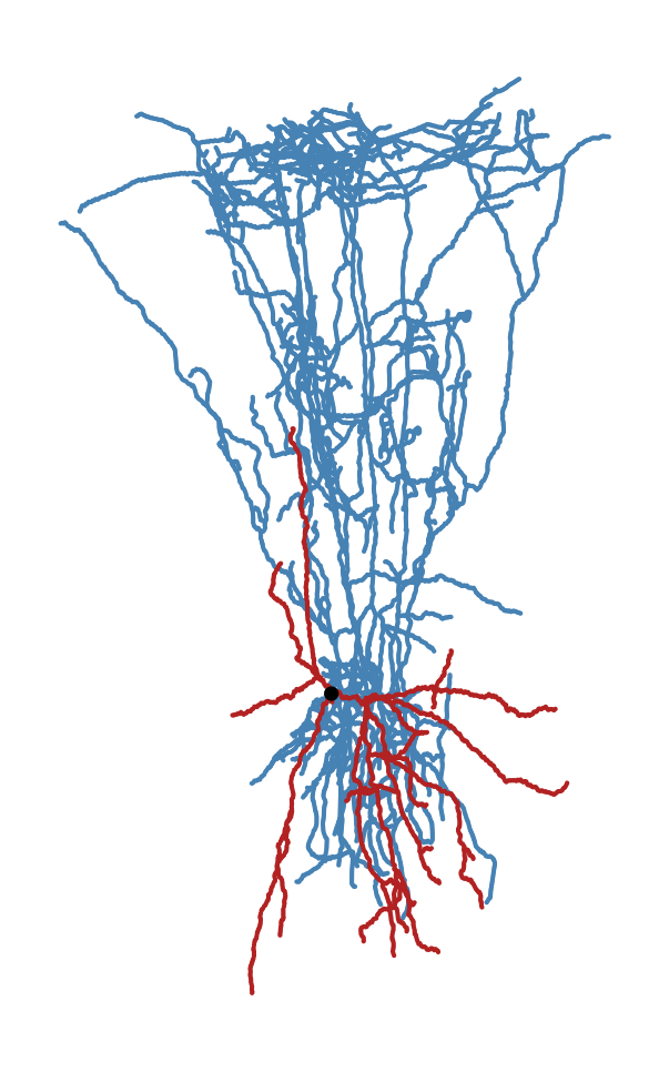
As an example, we will use an Sst+ inhibitory neuron from the Gouwens et al. (2020) study where we have also saved the layer drawings in the example_data directory as a JSON file in the format expected by skeleton_keys.

In its original orientation, the morphology looks like this:

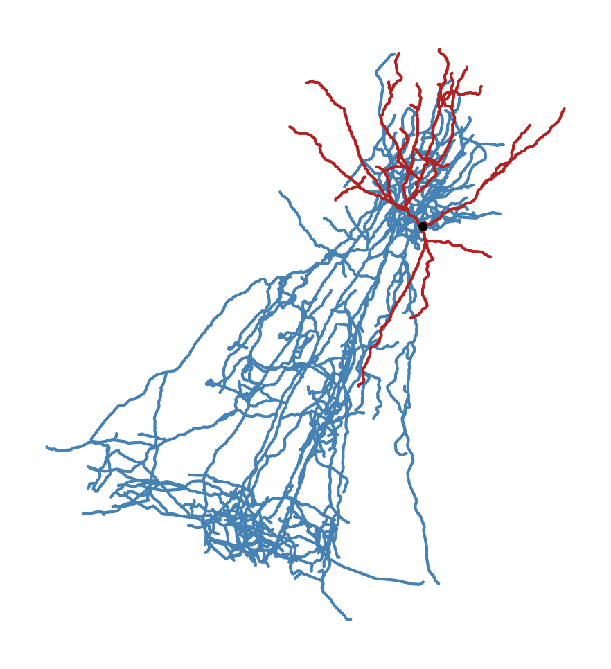
Sst neuron in original orientation. Dendrite is red, axon is blue, soma is black dot.

Our layer drawings (with a matched orientation) look like:

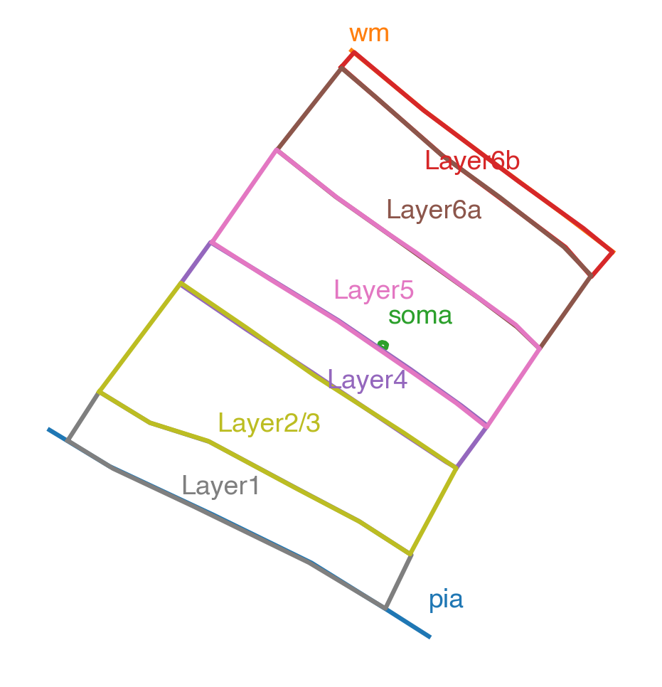
Pia, white matter, soma outline, and layer drawings

And together (after aligning the soma locations) they look like:

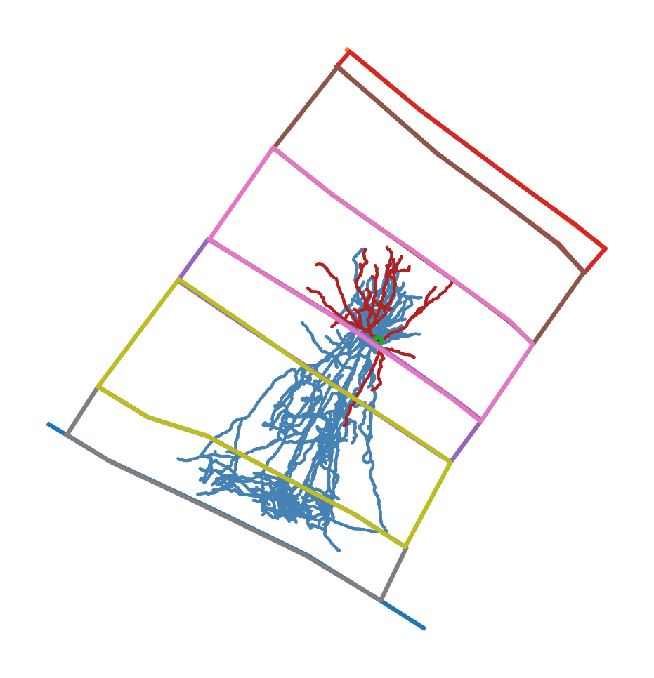
Morphology and layer drawings in original orientation

Note: This script also has functionality to correct the morphology for shrinkage (which can happen because the fixed tissue that is image dries out and becomes flatter than the original) and slice angle tilt (which happens when the cutting angle for brain slices does not match the curvature of that part of the brain). However, these features are currently written to require access to an internal Allen Institute database and do not yet have alternative input formats. Therefore, we will not use those functions in this guide.

We will supply the script with the following inputs:

• specimen_id - an integer identifier for the cell.

  Here, it is primarily used to access internal database information (which we aren’t doing), but in other scripts it is used to associate this cell with its features. Here, the specimen ID of our example is 740135032.

• swc_path - a file path to the SWC file in its original orientation.

  Here, our example cell’s SWC file is Sst-IRES-Cre_Ai14-408415.03.02.02_864876723_m.swc.

• surface_and_layers_file - a JSON file with the layer drawings.

  Here, our example uses the file 740135032_surfaces_and_layers.json.

• layer_depths_file - a JSON file with the set of layer depths we’re aligning the cell to.

  In this case we’ll use an average set of depths included as a test file, avg_layer_depths.json.

Therefore, our command will be:

skelekeys-layer-aligned-swc --specimen_id 740135032 \
--swc_path Sst-IRES-Cre_Ai14-408415.03.02.02_864876723_m.swc \
--surface_and_layers_file 740135032_surfaces_and_layers.json \
--layer_depths_file avg_layer_depths.json \
--correct_for_shrinkage False \
--correct_for_slice_angle False \
--output_file layer_aligned_740135032.swc

This creates a new SWC file (layer_aligned_740135032.swc) that is (1) uprighted and (2) stretched or squished to align each of its points to the reference set of layers.

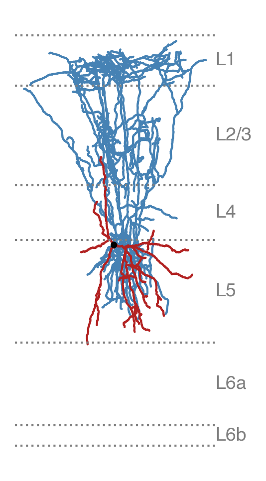
Layer-aligned morphology

Uprighting a morphology without layer alignment

If you only want to orient morphology so that pia is up and the white matter is down, but without making any layer thickness adjustments, you can use the command-line utility skelekeys-upright-corrected-swc. It still requires layer drawings, though, to know which direction the pia and white matter are relative to the originally reconstructed morphology.

Note: This script, too, can correct the morphology for shrinkage and slice angle tilt, but we are again skipping that since it currently can only use internally databased information.

It takes a similar set of arguments as before (but notably without the --layer_depths_file argument).

skelekeys-upright-corrected-swc --specimen_id 740135032 \
--swc_path Sst-IRES-Cre_Ai14-408415.03.02.02_864876723_m.swc \
--surface_and_layers_file 740135032_surfaces_and_layers.json \
--correct_for_shrinkage False \
--correct_for_slice_angle False \
--output_file upright_only_740135032.swc

The output looks like:

Upright (but not layer-aligned) morphology

Calculating depth profiles

A relevant aspect for distinguishing morphologies is the depth profile, which is a 1D histogram of the number of nodes across a set of depth bins, divided by compartment type (i.e., axon, basal dendrite, apical dendrite). These can be used to calculate reduced-dimesion representations of those profiles, determine the overlap of different compartment types, etc.

The command line utility skelekeys-profiles-from-swcs will create a CSV file of depth profiles from a list of layer-aligned SWC files.

The script expects the layer-aligned SWC files to be in a single directory (--swc_dir) and be named as {specimen_id}.swc. For this example, we have moved the layer-aligned Sst cell’s SWC file (740135032) into another directory and renamed it; we have also layer aligned a Pvalb cell (606271263) and a Vip cell (694146546).

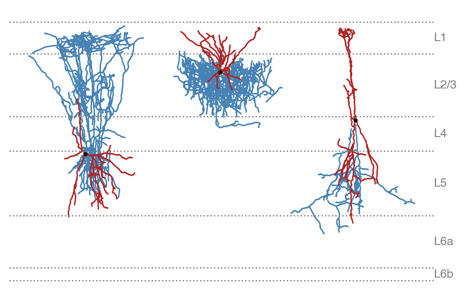
Layer-aligned Sst cell, Pvalb cell, and Vip cell

To run the script for our example, we give it the following inputs:

• specimen_id_file - a text file with specimen IDs

  The text file has one integer ID per line. Here we’re using example_specimen_ids.txt.

• swc_dir - the directory of layer-aligned SWC files

  Here our directory is layer_aligned_swcs

• layer_depths_file - a JSON file with the reference set of layer depths

  This is so that the script knows where the white matter begins (so that it can determine how far past to include)

• output_hist_file - an output CSV file path

  This CSV file contains the depth histograms - the columns are depth bins, and the rows are cells

• output_soma_file - an output CSV file path

  The script also saves the layer-aligned soma depths, which is used by other command line scripts in the package

Our command will then be:

skelekeys-profiles-from-swcs --specimen_id_file example_specimen_ids.txt \
--swc_dir layer_aligned_swcs \
--layer_depths_file avg_layer_depths.json \
--output_hist_file aligned_depth_profiles.csv \
--output_soma_file aligned_soma_depths.csv

This produces the following depth profiles:

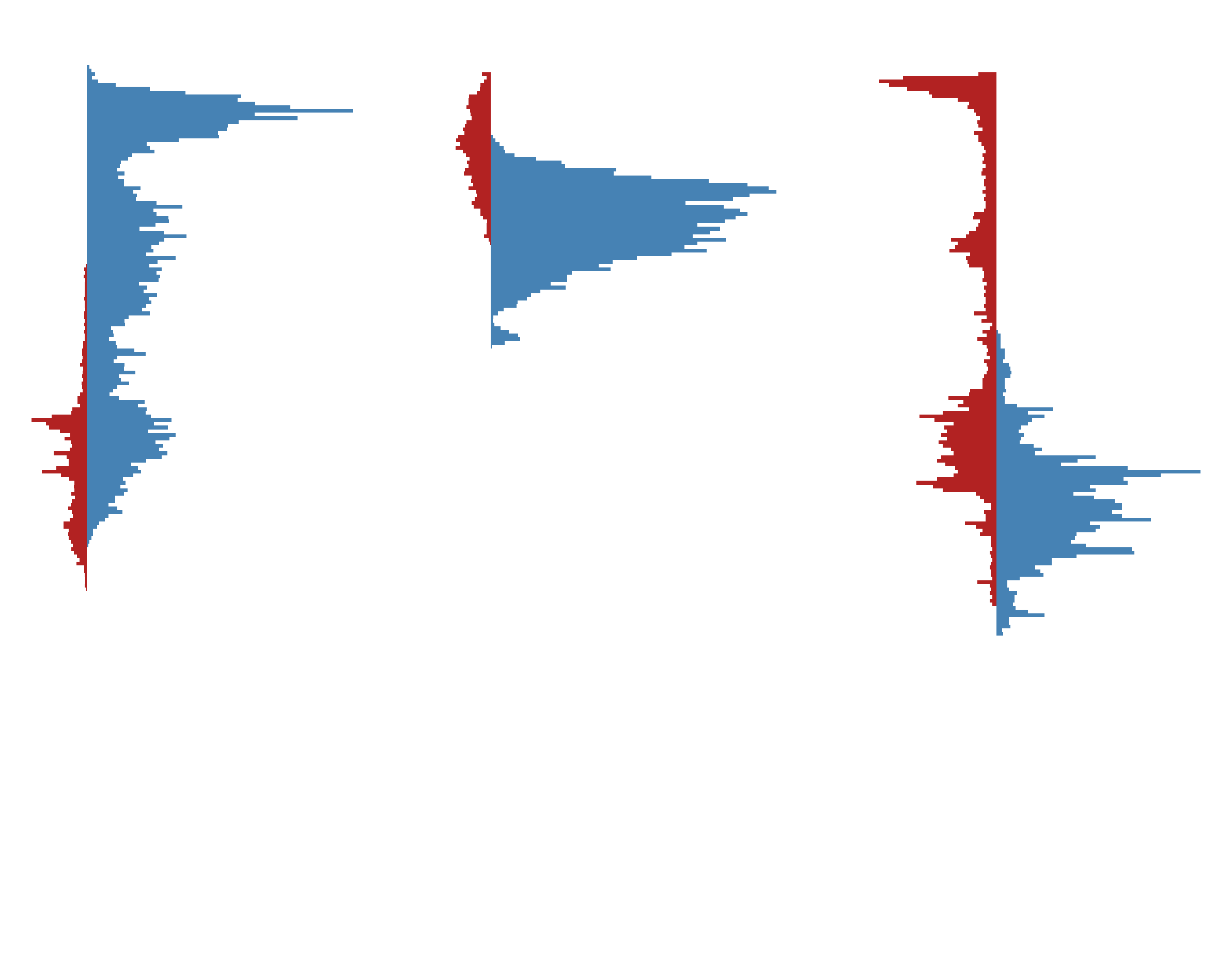
Layer-aligned depth profiles of the three example cells

PCA on depth profiles

A reduced dimension representation of the depth profiles can serve as useful features for distinguishing morphologies. However, analyses like PCA will produce loadings that vary depending on the data set. The command line utility skelekeys-calc-histogram-loadings can be used to generate a fixed loading file from a set of morphologies that can be used to analyze other morphologies with other scripts.

If you simply want to use the PCA loadings for a new set of cells and not transfer those loadings to another set, you do not need to use this utility (you can use the skelekeys-morph-features script by itself). That script will also let you save the loadings. But this script will allow you to calculate loadings without having to calculate all the other morphological features.

In this example, we will calculate and save the PCA loadings for the axonal compartments. The command to do so is:

skelekeys-calc-histogram-loadings --specimen_id_file example_specimen_ids.txt \
--aligned_depth_profile_file aligned_depth_profiles.csv \
--analyze_axon True \
--save_axon_depth_profile_loadings_file axon_loadings.csv

Calculating morphological features

Once we have the layer depths files (and optionally a set of pre-calculated loadings), we can calculate a set of morphological features for each cell using the command line utility skelekeys-morph-features. The main inputs are the set of upright (but not layer-aligned) SWC files and the depth profile CSV file. We also specify which compartments we want to analyze (for example if we have a set of excitatory neurons that don’t have reconstructed local axons, we would not want to analyze axonal compartments).

To continue our example, we will analyze the features using the following command:

skelekeys-morph-features  --specimen_id_file example_specimen_ids.txt \
--swc_dir upright_swcs \
--aligned_depth_profile_file aligned_depth_profiles.csv \
--aligned_soma_file aligned_soma_depths.csv \
--analyze_axon True \
--analyze_basal_dendrite True \
--analyze_apical_dendrite False \
--output_file example_features_long.csv

This produces a long-form feature data file.

Beginning of example long-form feature file

	specimen_id	feature	compartment_type	dimension	value
0	740135032	aligned_dist_from_pia	soma	none	488.95489922056464
1	606271263	aligned_dist_from_pia	soma	none	185.35510042590795
2	694146546	aligned_dist_from_pia	soma	none	363.1829539564272
3	740135032	depth_pc_0	axon	none	-591.3768052788041
4	740135032	depth_pc_1	axon	none	771.0611928161894
5	606271263	depth_pc_0	axon	none	1557.1882340570776
6	606271263	depth_pc_1	axon	none	-114.4320436027042
7	694146546	depth_pc_0	axon	none	-965.8114287782732
8	694146546	depth_pc_1	axon	none	-656.6291492134859
9	740135032	emd_with_basal_dendrite	axon	none	53.842009790570955
10	606271263	emd_with_basal_dendrite	axon	none	20.02095840833445
11	694146546	emd_with_basal_dendrite	axon	none	50.38248981181829
12	740135032	frac_above_basal_dendrite	axon	none	0.5537837260625045
13	740135032	frac_intersect_basal_dendrite	axon	none	0.4462162739374956
14	740135032	frac_below_basal_dendrite	axon	none	0.0
15	606271263	frac_above_basal_dendrite	axon	none	0.0
16	606271263	frac_intersect_basal_dendrite	axon	none	0.7648047321368555
17	606271263	frac_below_basal_dendrite	axon	none	0.23519526786314446
18	694146546	frac_above_basal_dendrite	axon	none	0.0
19	694146546	frac_intersect_basal_dendrite	axon	none	0.9692556634304207
20	694146546	frac_below_basal_dendrite	axon	none	0.030744336569579287
21	740135032	frac_above_axon	basal_dendrite	none	0.0
22	740135032	frac_intersect_axon	basal_dendrite	none	0.946916890080429
23	740135032	frac_below_axon	basal_dendrite	none	0.05308310991957105
24	606271263	frac_above_axon	basal_dendrite	none	0.37383177570093457
25	606271263	frac_intersect_axon	basal_dendrite	none	0.6261682242990654
26	606271263	frac_below_axon	basal_dendrite	none	0.0
27	694146546	frac_above_axon	basal_dendrite	none	0.47685185185185186
28	694146546	frac_intersect_axon	basal_dendrite	none	0.5231481481481481
29	694146546	frac_below_axon	basal_dendrite	none	0.0
30	740135032	extent	basal_dendrite	x	259.0984945349686
31	740135032	extent	basal_dendrite	y	360.15791867251323
32	740135032	bias	basal_dendrite	x	105.9123765215528
33	740135032	bias	basal_dendrite	y	-5.017693772805842

Post-processing morphological features

The long-form file can be used for many purposes, but it is also useful to convert the data to a wide format where the features are the columns and the rows are cells. At the same time, it can also be useful to normalize the different features for analyzes like classification and clustering.

The command line utility skelekeys-postprocess-features is used to perform these operations.

skelekeys-postprocess-features \
--input_files "['example_features_long.csv']" \
--wide_normalized_output_file example_features_wide_normalized.csv \
--wide_unnormalized_output_file example_features_wide_unnormalized.csv

Note the syntax for passing a list of files for the argschema command line argument. If you passed more than one file (for example, to normalize features calculated from two sets of cells to the same scale), you would separate each argument with a comma (as in "['file_one.csv','file_two.csv']").

The wide form feature file output looks like:

Example wide-form feature file

specimen_id	axon_bias_x	axon_bias_y	axon_depth_pc_0	axon_depth_pc_1	axon_emd_with_basal_dendrite	axon_exit_distance	axon_exit_theta	axon_extent_x	axon_extent_y	axon_frac_above_basal_dendrite	axon_frac_below_basal_dendrite	axon_frac_intersect_basal_dendrite	axon_max_branch_order	axon_max_euclidean_distance	axon_max_path_distance	axon_mean_contraction	axon_num_branches	axon_num_outer_bifurcations	axon_soma_percentile_x	axon_soma_percentile_y	axon_total_length	basal_dendrite_bias_x	basal_dendrite_bias_y	basal_dendrite_calculate_number_of_stems	basal_dendrite_extent_x	basal_dendrite_extent_y	basal_dendrite_frac_above_axon	basal_dendrite_frac_below_axon	basal_dendrite_frac_intersect_axon	basal_dendrite_max_branch_order	basal_dendrite_max_euclidean_distance	basal_dendrite_max_path_distance	basal_dendrite_mean_contraction	basal_dendrite_mean_diameter	basal_dendrite_num_branches	basal_dendrite_num_outer_bifurcations	basal_dendrite_soma_percentile_x	basal_dendrite_soma_percentile_y	basal_dendrite_stem_exit_down	basal_dendrite_stem_exit_side	basal_dendrite_stem_exit_up	basal_dendrite_total_length	basal_dendrite_total_surface_area	none_early_branch_path	soma_aligned_dist_from_pia	soma_surface_area
606271263	56.22872989248452	-121.2103061622121	1557.1882340570776	-114.4320436027042	20.02095840833445	0.0	0.6246170133542251	400.4118094004192	262.2553175261422	0.0	0.2351952678631444	0.7648047321368555	25.0	240.6846227360817	902.0221232091972	0.8194136640160532	665.0	1.845098040014257	0.4889426631713383	0.7447065940713854	16935.227964908227	0.1618829328459696	107.3874873605935	7.0	292.8979665049092	227.9213594244781	0.3738317757009345	0.0	0.6261682242990654	5.0	221.48224685084813	261.57785404864563	0.8777370205959968	0.5797508521165475	35.0	0.3010299956639812	0.4870808136338647	0.1423859263331501	0.4285714285714285	0.5714285714285714	0.0	2057.344684556989	3746.221348808403	0.5122275147209207	185.35510042590795	334.48341751636667
694146546	20.979837762279885	-337.62296125250555	-965.8114287782732	-656.6291492134859	50.38248981181829	8.953753130391712	0.8624144236833117	456.4507565320748	329.4824306809105	0.0	0.0307443365695792	0.9692556634304208	14.0	369.0094227941884	537.3808743109979	0.8804317016691116	117.0	1.462397997898956	0.3268608414239482	1.0	3856.927925804772	4.519987715724085	45.38310515181024	3.0	158.97060160570243	640.1652005614803	0.4768518518518518	0.0	0.5231481481481481	9.0	353.0402965262322	434.5470290069107	0.896216086452986	0.6016030092592592	69.0	1.1760912590556813	0.1689814814814815	0.5262345679012346	0.3333333333333333	0.0	0.6666666666666666	3185.736311407383	5983.0167307564	0.7175151344782787	363.1829539564272	240.61616017724623
740135032	5.169444355631811	297.6111166818944	-591.3768052788041	771.0611928161894	53.84200979057096	20.438908268544992	0.5210092861882935	424.4629900629744	587.2419117540196	0.5537837260625045	0.0	0.4462162739374956	24.0	465.7975422331148	712.7996048944084	0.8629205591762148	475.0	2.05307844348342	0.3885527158823948	0.1986189221897914	17053.86846302751	105.9123765215528	-5.017693772805842	4.0	259.0984945349686	360.15791867251323	0.0	0.053083109919571	0.946916890080429	9.0	196.6200075357029	228.6181419435221	0.8927636513643621	0.4823025201072386	44.0	0.7781512503836436	0.3179624664879356	0.8273458445040215	0.0	1.0	0.0	2204.244429816128	3338.8595673807986	0.9062144295279364	488.95489922056464	201.46425475133609

Working with general coordinates

The skeleton_keys package was originally built around processing SWC files, but it can also be used to align arbitrary sets of coordinates, if provided with the appropriate layer drawings.

The command line utility skelekeys-layer-aligned-coords can take a CSV and adjust the specified coordinates to make them layer-aligned. It takes the following inputs:

• coordinate_file - a CSV with coordinates

  The coordinate columns must contain “x”, “y”, and “z” in their names, but can have prefixes and/or suffixes (see below). We’ll use an example file named coord_example.csv.

• layer_depths_file a JSON file with the set of layer depths we’re aligning the cell to.

  Here again we’ll use an average set of depths included as a test file, avg_layer_depths.json.

• surface_and_layers_file - a JSON file with the layer drawings.

  Here, our example uses the file coord_layer_drawings.json.

• coordinate_column_prefix (and/or _suffix) - strings of common prefixes/suffixes

  This allows the coordinate columns to have names other than the default x, y, and z, but in this example we do not need to use them.

Using this, we can take a starting example file (the columns cell_id and target_cell_type contain extra metadata about the coordinates):

Example coordinate file

cell_id	target_cell_type	x	y	z
1	4P	838.184	691.792	821.64
1	4P	850.392	676.904	796.56
2	4P	741.704	649.608	737.76
3	5P-ET	739.656	680.464	950.92
3	5P-IT	762.28	748.584	826.44

Use the command:

skelekeys-layer-aligned-coords \
--coordinate_file coord_example.csv \
--surface_and_layers_file coord_layer_drawings.json \
--layer_depths_file avg_layer_depths.json \
--output_file aligned_coord_example.csv

And obtain:

Example coordinate file

cell_id	target_cell_type	x	y	z
1	4P	-92.0060469028378	-421.0797644340709	821.64
1	4P	-105.11025186647323	-399.30901042554444	796.56
2	4P	1.6844004295792985	-335.2109182277234	737.76
3	5P-ET	5.634215690400225	-382.48922026392205	950.92
3	5P-IT	-12.739372718728555	-508.88802416730545	826.44

Note that the x values have also changed because we have rotated the coordinates to an upright orientation (with pia at the top).

This aligned coordinate file can be used to generate histograms with the skelekeys-profiles-from-coords command line utility. You need to specify which column contains the depth values (here, the column labeled y) with the depth_label argument.

You can use other columns in the CSV file to split the histograms across rows using the --index_label argument, and/or you can create multiple histograms per row (as in the compartment type histograms above) with the --hist_split_label argument.

For example:

skelekeys-profiles-from-coords \
--coordinate_file aligned_coord_example.csv \
--layer_depths_file avg_layer_depths.json \
--depth_label y \
--index_label cell_id \
--hist_split_label target_cell_type \
--output_hist_file aligned_coord_hist.csv